Fast Timing-Conditioned Latent Audio Diffusion | Stability.AI
Jack Tol
2024-05-04
Section 1 - Introduction
1.1 - The Motivation
Generative AI is simply amazing:
- Text
- Images
- Video
- Audio
1.2 - Diffusion Models - What are they?
- A diffusion model is a type of generative machine learning model that gradually constructs data (images, video, audio) starting from a noisy distribution and progressively denoising it to produce complex samples.
- The model works by first adding noise to data over several steps to create a simple noise distribution, then learning to reverse this process to reconstruct the original data from the noise.
- During training, the model learns to predict the noise added to the data, rather than directly predicting the data itself.
1.3 - Diffusion Models - Conditioning
- Conditioning a diffusion model involves providing additional input, like text or labels, to guide the generation process towards a desired outcome.
- This conditioning allows for precise control over the features of the generated output, such as style, content, or specific attributes.
- To achieve this, modifications are made to the model’s architecture, training process, and input data to integrate and utilize the conditional data effectively.
1.4 - Diffusion Models - Applications
Applies to:
- Denoising
- Inpainting
- Super-resolution
- Image, Video, & Audio Generation
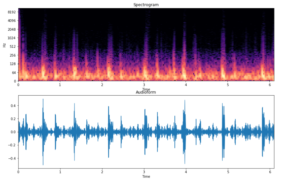
1.5 - Diffusion Models - The Type of Data We Use
![]()
![]()
Section 2 - Stable Audio Architecture
2.1 - Stable Audio Architecture
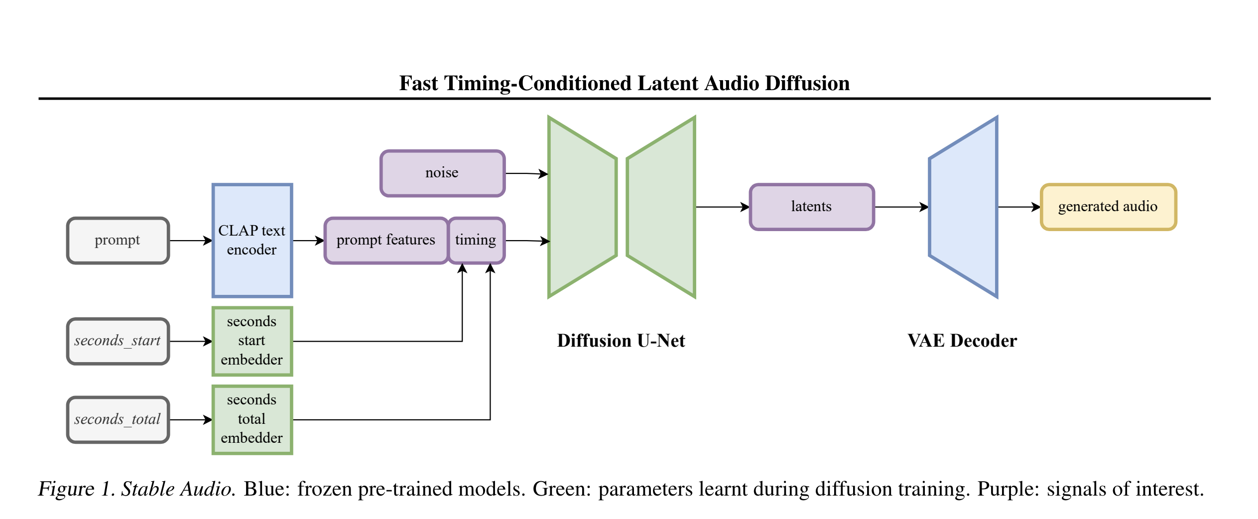
At the highest level, Stable Audio is a Latent Diffusion Model consisting of:
- Variational Autoencoder
- Conditioning Signals
- Diffusion Model
2.2 - Stable Audio Diagram
2.3 - Variational Autoencoder
- Faster Generation & Training Time
- Improved Audio Reconstruction at High Compression Ratios
- Trained From Scratch on Custom Dataset
- Downsamples Stereo Audio by a factor of 1024, Latent has 64 Dimensions
- Overall Compression Ratio of 32:1
2.3.1 - Variational Autoencoder Simple Diagram

2.3.2 - Variational Autoencoder Complex Diagram
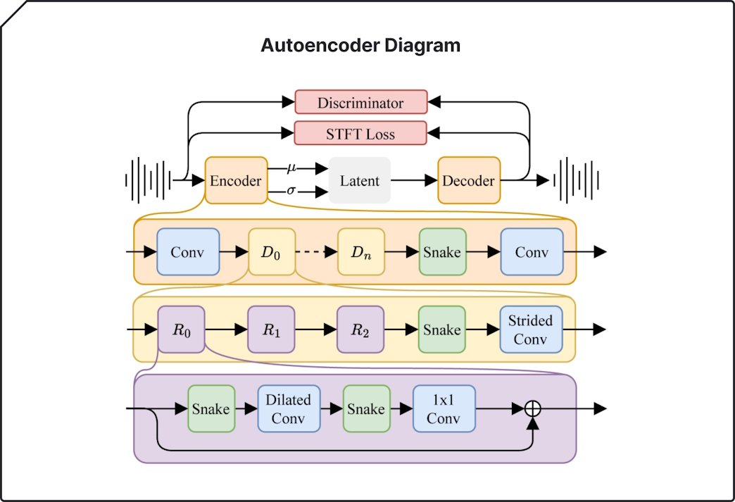
- Discriminator → Adversarial & Feature Matching Losses using STFT Loss
-
Each loss is weighted as follows:
- 1.0 for spectral losses
- 0.1 for adversarial losses
- 5.0 for the feature matching loss
- 1e-4 for the KL loss
- R0, R1, R2 → Residual Connections
- ⊕ → Summation Operator
- D1, Dn → Dilated Convolution
- Snake → Snake Activations
2.4 - Conditioning | CLAP Text Encoder
Acronyms
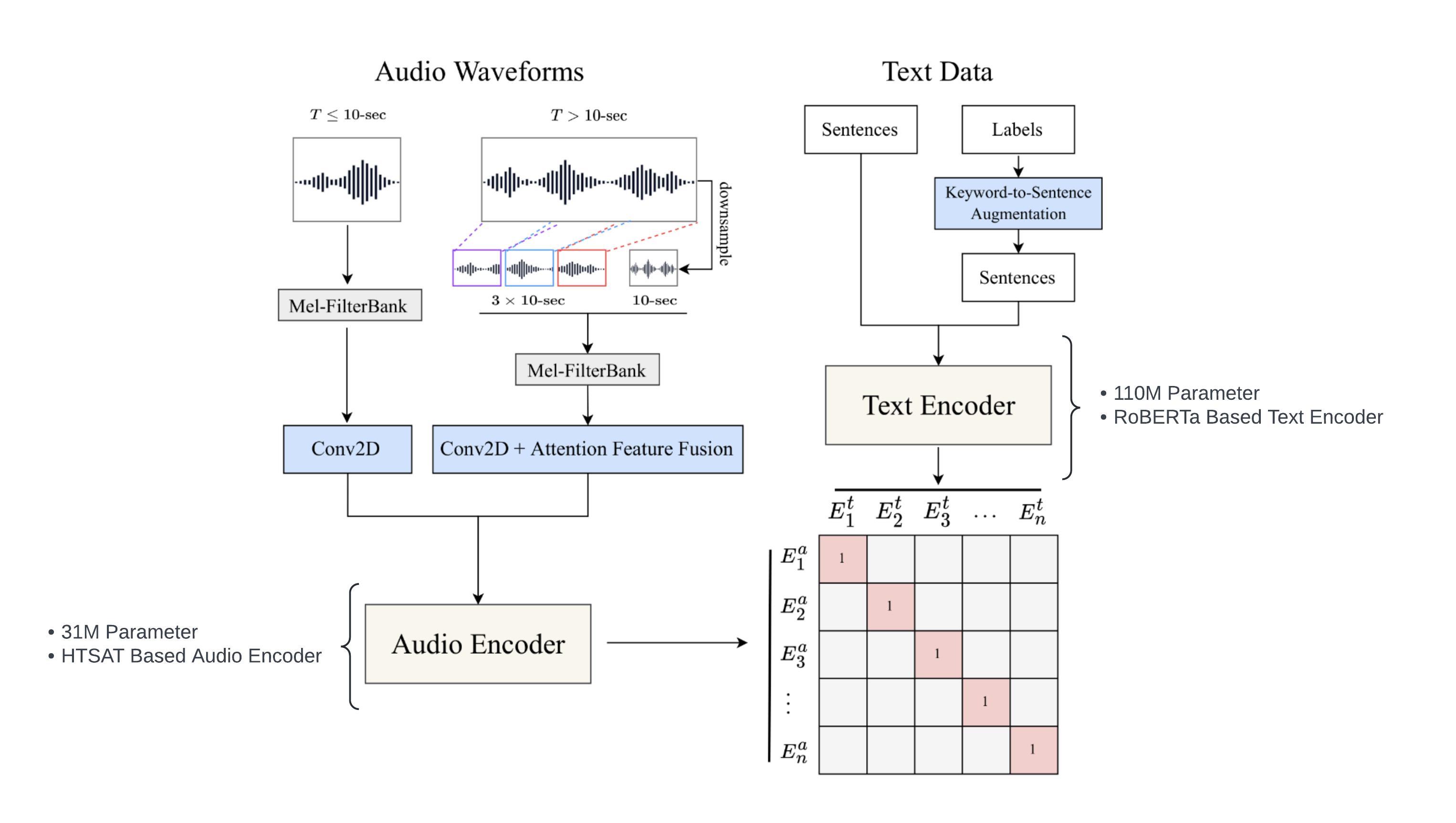
- CLAP - Contrastive Language-Audio Pretraining
- BERT - Bidirectional Encoder Representations from Transformers
- HTSAT - Hierarchical Token Semantic Audio Transformer
- RoBERTa - A Robustly Optimized BERT Pretraining Approach
2.4.1 - Conditioning | CLAP Text Encoder Diagram
2.4.2 - Conditioning | CLAP Text Encoder Cont.
- Trained From Scratch on Custom Dataset
- Both encoders trained using Language-Audio Contrastive Loss
- CLAP is used due to its native multimodality between words & audio
- Stable Audio’s CLAP Implementation can outperform the open-source CLAP and T5 embeddings models
- Uses the next-to-last layer to provide a better conditioning signal than the text features from the final layer
- These text features are provided to the diffusion U-Net through cross-attention layers
2.5 - Conditioning | Timing Embeddings
- Two Properties are Calculated when Gathering a Chunk of Audio from the Dataset:
- The second from which the chunk starts, denoted as seconds_start
- The number of seconds in the original audio file, denoted as seconds_total
These values are:
- Translated into per-second discrete learned embeddings
- Concatenated along the sequence dimension with text features derived from the prompt, providing a comprehensive context for processing
- And then, passed into the U-Net’s cross-attention layers
During inference, seconds_start and seconds_total serve as conditioning variables, enabling users to generate variable-length outputs.
When training with audio files shorter than the training window, padding with silence is used up to the training window length.
Suppose we take a 95-sec chunk from a 180-sec audio file, with the chunk starting 14-sec in, then:
- seconds_start = 14
- seconds_total = 180
2.5.1 - Conditioning | Timing Embeddings Diagram

2.6 - Diffusion Model Diagram
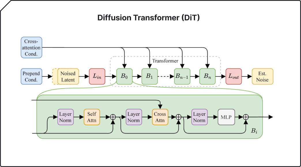
2.6.1 - Diffusion Model Cont.
- Based on a 907M parameter UNet
- 4 Levels of Symmetrical downsampling encoder blocks and upsampling decoder blocks
- Skip Connections added between encoder and decoder blocks
- The 4 levels have channel counts of 1024, 1024, 1024, and 1280, and downsample by factors of 1, 2, 2, and 4 respectively.
- Each encoder & decoder block has 3 attention layers
- The diffusion timestep conditioning is passed in through FiLM layers to modulate the model activations based on the noise level.
- Prompt & Timing Conditioning → Model through Cross Attention Layers
Section 3 - Training
3.1 - Dataset
806,284 Audio Samples totaling over 19,500 hours, consisting of:
- Music - 66% by Number of Files | 94% by Storage in GB’s
- Sound Effects - 25% by Number of Files | 5% by Storage in GB’s
- Instrument Stems - 9% by Number of Files | 1% by Storage in GB’s
With corresponding text metadata from AudioSparx.
3.2 - Variational Autoencoder
- Uses Automatic Mixed Precision for 1.1M steps
- Effective batch size of 256
- 16 A100 GPUs
- After 460,000 steps the encoder was frozen and the decoder was fine-tuned for an additional 640,000 steps
- Utilized multi-resolution sum and difference STFT loss for stereo signals with A-weighting before STFT, using window lengths of 2048, 1024, 512, 256, 128, 64, and 32. Weighted losses: 1.0 spectral, 0.1 adversarial, 5.0 feature matching, 1e-4 KL.
- Discriminators with STFT window lengths of 2048, 1024, 512, 256, and 128, use complex STFT representation and patch-based hinge loss.
3.3 - Text Encoder
- CLAP Model trained for 100 epochs from scratch on the custom dataset
- Effective batch size of 6,144
- 64 A100 GPUs
- CLAP Authors Setup
- Language-Audio Contrastive Loss
3.4 - Diffusion Model
- Exponential Moving Average & Automatic Mixed Precision for 640,000 steps
- 64 A100 GPUs
- Effective batch size of 256
- Resampled to 44.1kHz & sliced to 4,194,304 samples (95.1 sec)
- Longer files cropped, shorter files padded
- V-Objective with Cosine Noise Scheduler
- 10% Dropout on Conditioning Signals to be able to use Classifier-Free Guidance
- Text Encoder Frozen While Training the Diffusion Model
Section 4 - Methodology
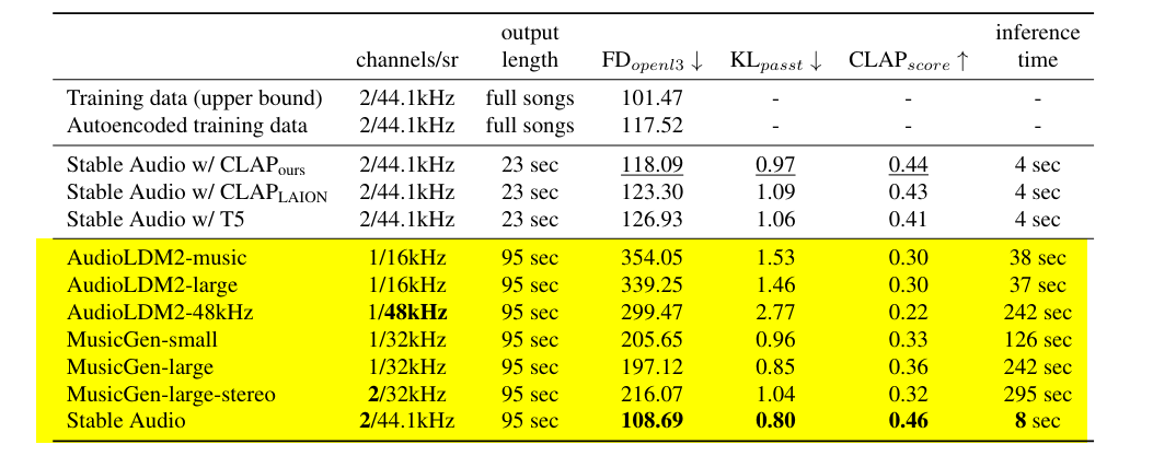
4.1 - Quantitative Metrics | \(FD_{Openl3}\)
- The Fréchet Distance (FD) measures the similarity between the statistics of generated and reference audio sets in a feature space.
- A low FD suggests that the generated audio closely matches the reference audio.
- Unlike the older VGGish method, which operates at 16 kHz, the \(Openl3\) feature space is used as it accepts signals up to 48 kHz, enhancing the ability to analyze high-quality audio.
- FD extended to evaluate stereo signals by independently processing left and right channels in the \(Openl3\) feature space, then concatenating them to create stereo features.
- This novel \(FD_{Openl3}\) metric allows more accurate assessments of higher quality, stereo audio content and is used.
4.2 - Quantitative Metrics | \(KL_{PaSST}\)
- PaSST is a state-of-the-art audio tagger trained on AudioSet used to compute the KL Divergence over the probabilities of labels between:
- Generated Audio
- Reference Audio
- The generated audio is expected to share similar semantics (tags) with the reference audio when the KL is low.
- The \(KL_{PaSST}\) is adapted to evaluate audio of varying lengths:
- Segmenting the audio into overlapping analysis windows
- Calculating the mean (across windows) of the generated logits and then applying a softmax
4.3 - Quantitative Metrics | \(CLAP_{score}\)
- The cosine similarity is computed between the \(CLAP_{LAION}\) text embedding of the given text prompt and the \(CLAP_{LAION}\) audio embedding of the generated audio.
- A high \(CLAP_{score}\) denotes that the generated audio adheres to the given text prompt.
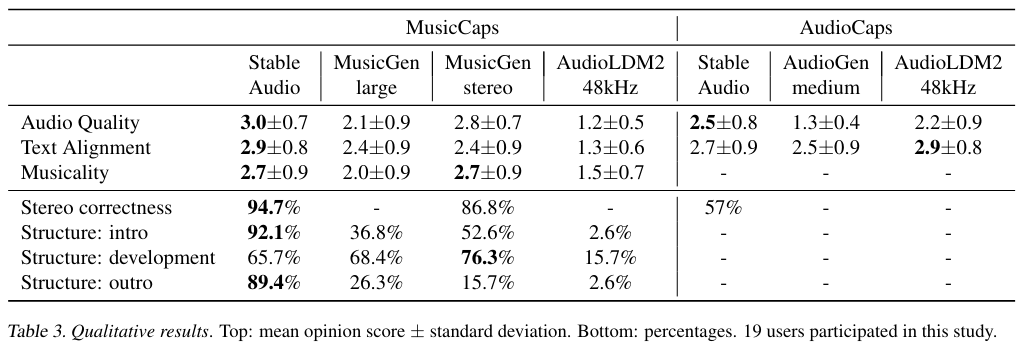
4.4 - Qualitative Metrics
- Audio Quality - Evaluates whether the generated audio is of low-fidelity with artifacts or high-fidelity.
- Text Alignment - Evaluates how the generated audio adheres to the given text prompt.
- Musicality (music only) - Evaluates the capacity of the model to articulate melodies and harmonies.
- Stereo Correctness (stereo only) - Evaluates the appropriateness of the generated spatial image.
- Musical Structure (music only) - Evaluates if the generated song contains intro, development, and/or outro.
Human Ratings Collected:
- 0 | Bad
- 1 | Poor
- 2 | Fair
- 3 | Good
- 4 | Excellent
4.5 - Evaluation Data | Experiments
- MusicCaps & AudioCaps standard benchmarks are used.
- MusicCaps contains 5521 music segments from YouTube, each with 1 caption.
- AudioCaps contains 979 audio segments from YouTube, each with several captions.
- For each model tested, an audio is generated per caption (5521 for MC & 4875 for AC).
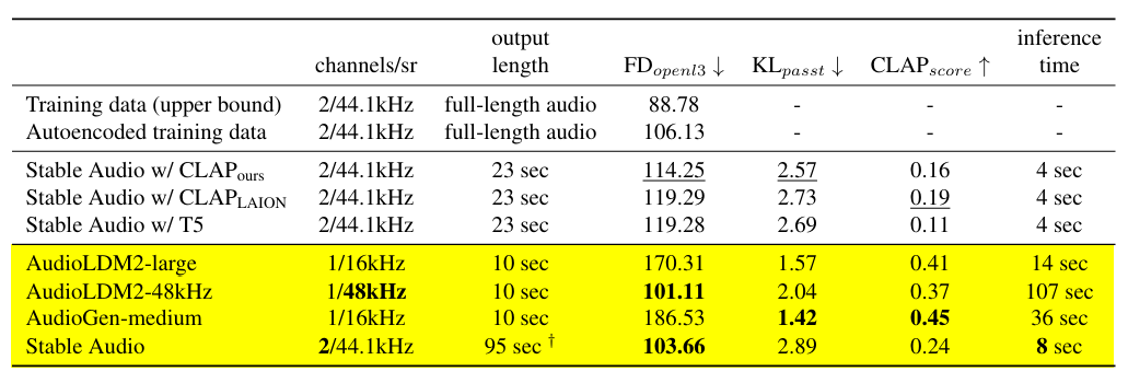
- MC & AC only represent 10 sec segments of audio, therefore, the full-length audios were also considered.
- However, results do not hold consistently due to the label only accurately representing the 10 sec audios, while the generated audio ranged from 10 sec to 95 secs.
4.6 - Evaluation Data | Qualitative Experiments
- Prompts for were randomly picked from MusicCaps and AudioCaps.
- Avoided captions which included “low quality” or a similar phrase to focus on high-fidelity synthesis.
- Avoided ambient music because users found it challenging to evaluate musicality.
- Avoided speech-related prompts since it was out of focus.
4.7 - Evaluation Data | Quantitative Results on MusicCaps
4.8 - Evaluation Data | Quantitative Results on AudioCaps
4.9 - Evaluation Data | Qualitative Results on Both MusicCaps & AudioCaps
Section 5 - Experiments
5.1 - How does the autoencoder impact audio fidelity?
Stable Audio VAE Reconstruction Demo
MusicCaps

AudioCaps

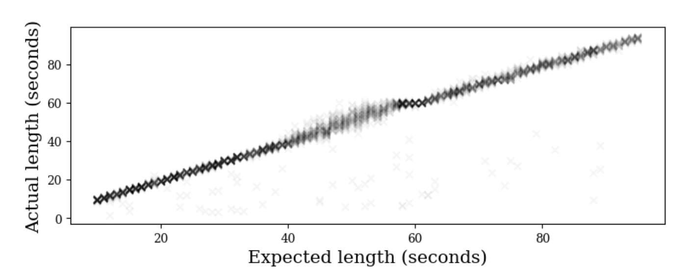
5.2 - How accurate is the timing conditioning?
- The model consistently produces audio matching the expected lengths.
- Increased errors occur in the 40-60 seconds range due to less training data.
- Audio length is measured using a basic energy threshold to detect silence.
- Shortest lengths may be inaccurately short due to limitations in the silence detection method.
Section 6 - Conclusion
Conclusion
- Enables the rapid generation of variable-length, long-form stereo music and sounds at 44.1kHz from textual and timing inputs.
- Novel qualitative and quantitative metrics were used for evaluating long-form full-band stereo signals, and found Stable Audio to be a top contender, if not the top performer, in two public benchmarks.
- Differently from other state-of-the-art models, Stable Audio can generate music with structure and stereo sound effects.